Recently, I spent sometime writing out the code for a neural network in python from scratch, without using any machine learning libraries. It proved to be a pretty enriching experience and taught me a lot about how neural networks work, and what we can do to make them work better. I thought I’d share some of my thoughts in this post.

Defining the Learning Problem

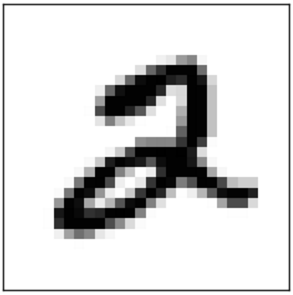
In supervised learning problems, we’re given a training dataset that contains pairs of input instances and their corresponding labels. For example, in the MNIST dataset, our input instances are images of handwritten digits, and our labels are a single digit that indicate the number written in the image. To input this training data to a computer, we need to numerically represent our data. Each image in the MNIST dataset is a 28 x 28 grayscale image, so we can represent each image as a vector \(\vec{x} \in R^{784}\). The elements in the vector \(x\) are known as features, and in this case they’re values in between 0 and 255. Our labels are commonly denoted as \(y\), and as mentioned, are in between 0 and 9. Here’s an an example from the MNIST dataset [1]:

We can think of this dataset as a sample from some probability distribution over the feature/label space, known as the data generating distribution. Specifically, this distribution gives us the probability of observing any particular \((x, y)\) pairs for all \((x, y)\) pairs in the cartesian product \(X \cdot Y\). Intuitively, we would expect that the pair that consists of an image of a handwritten 2 and the label 2 to have a high probablity, while a pair that consists of a handwritten 2 and the label 9 to have a low probability.

Unfortunately, we don’t know what this data generating distribution is parametrized by, and this is where machine learning comes in: we aim to learn a function \(h\) that maps feature vectors to labels as accurately as possible, and in doing so, come up with estimates for the true underlying parameters. This function should generalize well: we don’t just want to learn a function that produces a flawless mapping on our training set. The function needs to be able to generalize over all unseen examples in the distribution. With this, we can introduce the idea of the loss function, a function that quantifies how off our prediction is from the true value. The loss function gives us a good idea about our model’s performance, so over the entire population of (feature vector, label) pairs, we’d want the expectation of the loss to be as low as possible. Therefore, we want to find \(h(x)\) that minimizes the following function:

However, there’s a problem here: we can’t compute \(p(x, y)\), so we have to resort to approximations of the loss function based on the training data that we do have access to. To approximate our loss, it is common to sum the loss function’s output across our training data, and then divide it by the number of training examples to obtain an average loss, known as the training loss:

There are several different loss functions that we can use in our neural network to give us an idea of how well it is doing. The function that I ended up using was the cross-entropy loss, which will be discussed a bit later.

In the space of neural networks, the function \(h(x)\) we will find will consist of several operations of matrix multiplications followed by applying nonlinearity functions. The basic idea is that we need to find the parameters of this function that both produce a low training loss and generalize well to unseen data. With our learning problem defined, we can get on to the theory behind neural networks:

Precursor: A single Neuron

In the special case of binary classification, we can model an artificial neuron as receiving a linear combination of our inputs \(w^{T} \cdot x\), and then computing a function that returns either 0 or 1, which is the predicted label of the input.

The weights are applied to the inputs, which are just the features of the training instance. Then, as a simple example of a function an artificial neuron can compute, we take the sign of the resulting number, and map that to a prediction. So the following is the neural model of learning [2]:

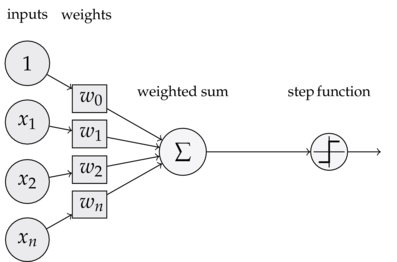
There’s a few evident limitations to this kind of learning - for one, it can only do binary classification. Moreover, this neuron can only linearly separate data, and therefore this model assumes that the data is indeed linearly separable. Deep neural networks are capable of learning representations that model the nonlinearity inherent in many data samples. The idea, however, is that neural networks are just made up of layers of these neurons, which by themselves, are pretty simple, but extremely powerful when they are combined.

From Binary Classification to Multinomial Classfication

In the context of our MNIST problem, we’re interested in producing more than a binary classification - we want to predict one label out of a possible ten. One intuitive way of doing this is simply training several classifiers - a one classifier, a two classifier, and so on. We don’t want to train multiple models separately though, we’d like a single model to learn all the possible different classifications.

If we consider our basic model of a neuron, we see that it has one vector of weights that it applies to determine a label. What if we had multiple vectors - a matrix - of weights instead? Then, each row of weights could represent a separate classifier. To see this clearly, we can start off with a simple linear mapping:

For our MNIST problem, x is a vector with 784 components, W was originally a single vector with 784 values, and the bias, b, was a single number. However, if we modified W to be a matrix instead, we get multiple rows of weights, each of which can be applied to the input x via a matrix multiplication. Since we want to be able to predict 10 different labels, we can let W be a 10 x 784 matrix, and the matrix product \(Wx\) will produce a column vector of values that represent the output of 10 separate classifiers, where the weights for each classifier is given by the rows of W. The bias term is now a 10-dimensional vector that each add a bias term to matrix product. The core idea, however, is that this matrix of weights represent different classifiers, and now we can predict more than just binary labels. An image from Stanford’s CS 231n course shows this clearly [3]:

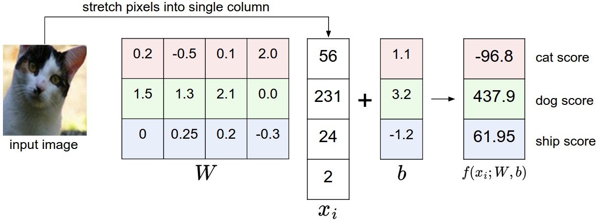
Now that we have a vector of outputs that roughly correspond to scores for each predicted class, we’d like to figure out the most likely label. To do this, we can map our 10 dimensional vector to another 10 dimensional vector which each value is in the range (0, 1), and the sum of all values is 1. This is known as the softmax function. We can use the output of this function to represent a probability distribution: each value gives us the probability of the input x mapping to a particular label y. The softmax function’s input and output are both vectors, and it can be defined as \(\frac{e^{z_i}}{\sum_{i=1}^{N} e^{z_i}}\)

Next, we can use our loss function discussed previously to evaluate how well our classifier is doing. Specifically, we use the cross-entropy loss, which for a single prediction/label pair, is given by \(C(S,L) = - \sum_{i}L_{i}log(S_{i})\).

Here, \(L\) is a specific one-hot encoded label vector, meaning that it is a column vector that has a 1 at the index corresponding to its label, and is zero everywhere else. \(S\) is a prediction vector whose elements sum to 1. As an example, we may have:

The contribution to the entire training data’s loss by this pair was 0.70. To contrast, we can swap the first two probabilities in our softmax vector. We then end up with a lower loss:

So our cross-entropy loss makes intuitive sense: it is lower when our softmax vector has a high probability at the index of the true label, and it is higher when our probabilities indicate a wrong or uncertain choice. The average cross entropy loss is given by plugging into the average training loss function given above. A large part of training our neural network will be finding parameters that make the value of this function as small as possible, but still ensuring that our parameters generalize well to unseen data. For the linear softmax classifier, the training loss can be written as:

This is the function that we seek to minimize. Using the gradient descent algorithm, we can learn a particular matrix of weights that performs well and produces a low training loss. The assumption is that a low trainin gloss will correspond to a low expected loss across all samples in the population of data, but this is a risky assumption that can lead to overfitting. Therefore, a lot of research into machine learning is directed towards figuring out how to minimize training loss while also retaining the ability to generalize.

Now that we’ve figured out how to linearly model multilabel classification, we can create a basic neural network. Consider what happens when we combine the idea of artificial neurons with our logistic classifier. Instead of computing a linear function \(Wx + b\) and immediately passing the result to a softmax function, we can have an intermediate step: pass the output of our linear combination to a vector of artificial neurons, that each compute a nonlinear function. Then, we can take a linear combination with a vector of weights for each of these outputs, and pass that into our softmax function.

Our previous linear function was given by:

And our new function is not too different:

The key differences are that we have more biases and weights, as well as a larger composition of functions. This function is harder to optimize, and introduces a few interesting ideas about learning the weights with an algorithm known as backpropagation.

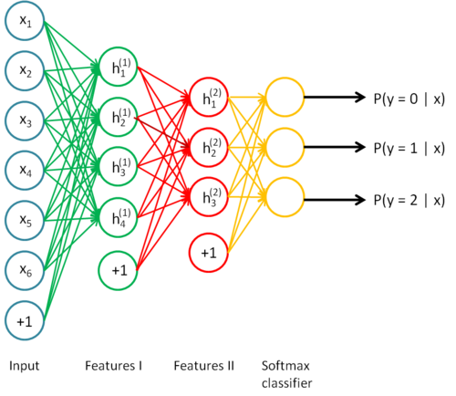
This “intermediate step” is actually known as a hidden layer, and we have complete control over it, meaning that among other things, we can vary the number of parameters or connections between weights and neurons to obtain an optimal network. It’s also important to notice that we can stack an arbitrary amount of these hidden layers between the input and output of our network, and we can tune these layers individually. This lets us make our network as deep as we want it. For example, here’s what a neural network with two hidden layers would look like [4]:

Implementing the Neural Network

With a bit of background out of the way, we can actually begin implementing our network. If we’re going to implement a neural network with one hidden layer of arbitrary size, we need to initalize two matrices of weights: one to multiply with our inputs to feed into the hidden layer, and one to multiply with the outputs of our hidden layer, to feed into the softmax layer. Here’s how we can initialize our weights:

import numpy as np
def init_weights(num_input_features, num_hidden_units, num_output_units):
    """initialize weights uniformly randomly with small values"""
    w1 = np.random.uniform(-1.0, 1.0, size=num_hidden_units*(num_input_features + 1)
                          ).reshape(num_hidden_units, num_input_features + 1)
    w2 = np.random.uniform(-1.0, 1.0, size=num_output_units*(num_hidden_units+1)).reshape(num_output_units, num_hidden_units+ 1)
    return w1, w2
w1, w2 = init_weights(784, 30, 10)
print w1.shape # expect 
print w2.shape # expect

(30, 785)
(10, 31)

An important preprocessing step is to one-hot encode all of our labels. This is a typical process in machine learning and deep learning problems that involve modeling more labels than two. We begin with a 1-dimensional vector \(y\) with m elements, where element \(y_i \in [0...N]\) and turn it into an N x M matrix Y. Then, the ith column in Y represents the ith training label (this is also the element at index i in \(y_i\)). For this column, the label is given by the element j for which the value \(Y[j][i] = 1\).

In other words, we’ve taken a vector in which a label j is given by \(y[i] = j\) and changed it into the matrix where the label would be j for the ith training example if \(Y[j][i] = 1\). From this, we can implement a one-hot encoding:

def encode_labels(y, num_labels):
        """ Encode labels into a one-hot representation
            Params:
            y: numpy array of num_samples, contains the target class labels for each training example.
            For example, y = [2, 1, 3, 3] -> 4 training samples, and the ith sample has label y[i]
            k: number of output labels
            returns: onehot, a matrix of labels by samples. For each column, the ith index will be
            "hot", or 1, to represent that index being the label.
        """
        onehot = np.zeros((num_labels, y.shape[0]))
        for i in range(y.shape[0]):
            onehot[y[i], i] = 1.0
        return onehot
    
y_train = np.array([0,1,8,7,4,5,0,1,4])
Y = encode_labels(y_train,9)
Y

array([[ 1.,  0.,  0.,  0.,  0.,  0.,  1.,  0.,  0.],
       [ 0.,  1.,  0.,  0.,  0.,  0.,  0.,  1.,  0.],
       [ 0.,  0.,  0.,  0.,  0.,  0.,  0.,  0.,  0.],
       [ 0.,  0.,  0.,  0.,  0.,  0.,  0.,  0.,  0.],
       [ 0.,  0.,  0.,  0.,  1.,  0.,  0.,  0.,  1.],
       [ 0.,  0.,  0.,  0.,  0.,  1.,  0.,  0.,  0.],
       [ 0.,  0.,  0.,  0.,  0.,  0.,  0.,  0.,  0.],
       [ 0.,  0.,  0.,  1.,  0.,  0.,  0.,  0.,  0.],
       [ 0.,  0.,  1.,  0.,  0.,  0.,  0.,  0.,  0.]])

With that out of the way, we’re ready to start implementing the bread and butter of the neural network: the fit() function. Fitting a function to our data requires two key steps: the forward propagation, where we make a prediction for a specific training example, and the backpropagation algorithm, where we update each of our weights by calculating the weight’s impact on our prediction error. The prediction error is quantified by the average training loss discussed above.

The first step in implementing the entire fit function will be to implement forward propagation. I decided to use the tanh function as the nonlinearity. Other popular choices include the sigmoid and ReLu functions. The forward propagation code passes our inputs to the hidden layer via a matrix multiplication with weights, and the output of the hidden layer is multiplied with a different set of weights, the result of which is passed into the softmax layer from which we obtain our predictions.

It’s also useful to save and return these intermediate values instead of only returning the prediction, since we’ll need these values later for backpropagation.

def forward(X, w1, w2, do_dropout = True):
        """ Compute feedforward step """
        #the activation of the input layer is simply the input matrix plus bias unit, added for each sample.
        a1 = add_bias_unit(X)
        #the input of the hidden layer is obtained by applying our weights to our inputs. We essentially take a linear combination of our inputs
        z2 = w1.dot(a1.T)
        #applies the tanh function to obtain the input mapped to a distrubution of values between -1 and 1
        a2 = self.tanh(z2)
        #add a bias unit to activation of the hidden layer.
        a2 = self.add_bias_unit(a2, column=False)
        # compute input of output layer in exactly the same manner.
        z3 = w2.dot(a2)
        # the activation of our output layer is just the softmax function.
        a3 = self.softmax(z3)
        return a1, z2, a2, z3, a3

Since these operations are all vectorized, we generally run forward propagation on the entire matrix of training data at once. Next, we want to quantify how “off” our weights are, baed on what was predicted. The cost function is given by \(-\sum_{i,j} L_{i,j}log(S_{i,j})\) , where \(L\) is the one-hot encoded label for a particular example and \(S\) is the output of the softmax function in the final layer of our neural network. In code, it can be implemented as follows:

def get_cost(self, y_enc, output, w1, w2):
        """ Compute the cost function."""
        cost = - np.sum(y_enc*np.log(output))
        cost = cost
        return cost/y_enc.shape[1] #average cost

Learning Weights with Gradient Descent

Now we’re at a stage where our neural network can make predictions given training data, compare it to the actual labels, and quantify the error across our entire training dataset. Our network is able to learn quite yet however. The actual “learning” happens with the gradient descent algorithm. Gradient descent works by computing the partial derivative of our weights with respect to the cost. The vector of these partial derivatives gives us the direction of fastest increase for our loss function (in particular, it can be shown mathematically that the gradient of a function points in the direction of fastest increase). Then, we update each of our weights by the negative value of the gradient (hence the “descent” part of gradient descent. This can be seen as taking a “step” in the direction of a minimum. The size of this step is given by a hyperparameter known as the learning rate, which turns out to be extremely important in getting gradient descent to work. In general, the gradient descent algorithm can be given as follows:

while not converged:

Gradient descent seeks to find the weights that bring our cost function to a global minimum. Intuitively, this makes sense, as we’d like our cost function to be as low as possible (while still taking care not to overfit on our training data). However, the functions that quantify the loss for most machine learning algorithms tend not to have an explicit solution to \(\frac{\delta L}{\delta W} = 0\), so we must use numerical optimization algorithms such as gradient descent to hopefully get to a local minimum. It turns out that we’re not always gauranteed to get to a global minimum either. Gradient descent only converges to a global minimum if our cost function is convex, and while cost functions for algorithms such as logistic regression are convex, the cost function for our single hidden layer neural network is not.

We can still use gradient descent and get to a reasonably good set of weights, however. The art of doing this is an active area of deep learning research. Currently, a common method for implementing gradient descent for deep learning seems to be:

1) Initializing your weights sensibly. This often involves some experimentation in how you initialize your weights. If your network is not very deep, initializing them randomly with small values and low variance usually works. If your network is deeper, larger values are preferred. Xavier initialization is a useful algorithm that determines weight initialization with respect to the net’s size.

2) Choosing an optimal learning rate. If the learning rate is too large, gradient descent could end up actually diverging, or skipping over the minimum entirely since it takes steps that are too large. Likewise, if the learning rate is too small, gradient descent will converge much more slowly. In general, it is advisable to start off with a small learning rate and decay it over time as your function begins to converge.

3) Use minibatch gradient descent. Instead of computing the loss and weight updates across the entire set of training examples, randomly chooose a subset of your training examples and use that to update your weights. While this may cause gradient descent to not work optimally at each iteration, it is much more efficient so we end up winning by a lot. We essentially approximate the gradient across the entire training set from a sample from the training set.

4) Use the momentum method. This involves remembering the previous gradients, and factoring in the direction of those previous gradients when calculating the current update. This has proved to be pretty successful, as Geoffrey Hinton discusses in this video.

As a side note, the co-founder of OpenAI, Ilya Sutskever, has more about training deep neural networks with stochastic gradient descent here

Here’s an implementation of the fit() function:

def fit(self, X, y, print_progress=True):
        """ Learn weights from training data """
        X_data, y_data = X.copy(), y.copy()
        y_enc = self.encode_labels(y, self.n_output)
        # init previous gradients
        prev_grad_w1 = np.zeros(self.w1.shape)
        prev_grad_w2 = np.zeros(self.w2.shape)

        #pass through the dataset
        for i in range(self.epochs):
            self.learning_rate /= (1 + self.decay_rate*i)
            # use minibatches
            mini = np.array_split(range(y_data.shape[0]), self.minibatch_size)
            for idx in mini:
                #feed feedforward
                a1, z2, a2, z3, a3= self.forward(X_data[idx], self.w1, self.w2)
                cost = self.get_cost(y_enc=y_enc[:, idx], output=a3, w1=self.w1, w2=self.w2)

                #compute gradient via backpropagation
                grad1, grad2 = self.backprop(a1=a1, a2=a2, a3=a3, z2=z2, y_enc=y_enc[:, idx], w1=self.w1, w2=self.w2)
                # update parameters, multiplying by learning rate + momentum constants
                # gradient update: w += -alpha * gradient.
                w1_update, w2_update = self.learning_rate*grad1, self.learning_rate*grad2
                # gradient update: w += -alpha * gradient.
                # use momentum - add in previous gradient mutliplied by a momentum hyperparameter.
                momentum_factor_w1 = self.momentum_const * prev_grad_w1
                momentum_factor_w2 = self.momentum_const * prev_grad_w2
                
                #update
                self.w1 += -(w1_update + momentum_factor_w1)
                self.w2 += -(w2_update + momentum_factor_w2)

                # save current gradients
                prev_grad_w1, prev_grad_w2 = w1_update, w2_update

            if print_progress and (i+1) % 50==0:
                print "Epoch: " + str(i+1)
                print "Loss: " + str(cost)
                acc = self.training_acc(X, y)
                print "Training Accuracy: " + str(acc)

        return self

To compute the actual gradients, we use the backpropagation algorithm that calculates the gradients that we need to update our weights from the outputs of our feed forward step. Essentially, we repeatedly apply the chain rule starting from our outputs until we end up with values for \(\frac{\delta L}{\delta W_1}\) and \(\frac{\delta L}{\delta W_2}\). CS 231N provides an excellent explanation of backprop.

Our forward pass was given by:

a1 = X
z2 = w1  * a1.T
a2 = tanh(z2)
z3 = w2 * a1
a3 = softmax(z3)

Using these values, our backwards pass can be given by:

s3 = a3 - y_actual
grad_w1 = s3 * a2
s2 = w2.T * s3 * tanh(z2, deriv=True)
grad_w2 = s3 * a2.T

The results of our backwards pass were used in the fit() function to update our weights. That’s essentially all of the important parts of implementing a neural network, and training this vanilla neural network on MNIST with 1000 epochs gave me about 95% accuracy on test data. There’s still a few more bells and whistles we can add to our network to make it generalize better to unseen data, however. These techniques reduce overfitting, and two common ones are L2-regularization and dropout.

L2-regularization

Using L2-regularization in neural networks is the most common way to address the issue of overfitting. L2 regularization adds a term to the cost function which we seek to minimize.

Previously, our cost function was given by \(- \sum_{i,j} L_{i,j} log(S_{i,j})\)

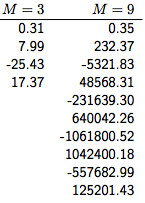
Now, we tack on an additional regularization term: \(0.5 \lambda W^{2}\). Essentially, we impose a penalty on large weight values. Large weights are indicative of overfitting, so we want to keep the weights in our model relatively small, which is more indicative of a simpler model. To see why this is, consider the classic case of overfitting, where our learning algorithm essentially memorizes the training data [5]:

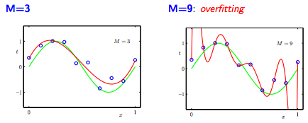
The values for the degree 9 polynomial are much greater than the values for the degree 3 polynomial:

With regularization, when we minimize the cost function, we have two separate goals. Minimizing the first term picks weight values that give us the smallest training error. Minimizing the second term picks weight values that are as small as possible. The value of the hyperparameter \(\lambda\) controls how much we penalize large weights: if \(\lambda\) is 0, we don’t regularize at all, and if \(\lambda\) is very large, then the entropy term becomes ignored and we prioritize small weight values.

Adding the L2-regularization term to the cost function does not change gradient descent very much. The derivative with respect to \(W\) with of to the regularization term \(0.5 \lambda W^2\) is simply \(\lambda W\), so we just add that term while computing the gradient. The result of adding this extra term to the gradients is that each time we update our weights, the weights undergo a linear decay.

While L2-regularization is quite popular, a few other forms of regularization are used as well. Another common method is L1-regularization, in which we add on the L1-norm of our weights, multiplied by the regularization hyperparameter: \(\lambda W\).

With L1-regularization, we penalize weights that are non-zero, thus leading our network to learn sparse vectors of weights (vectors where many of the weight entries are zero). Therefore, our neurons will only fire when the most important features (whatever they may be) are detected in our training examples. This helps with feature selection.

Dropout

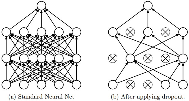
Dropout is a recently introduced, but very effective technique for reducing overfitting in neural networks. Generally, every neuron in a particular layer is connected to all the neurons in the next layer. This is called a “fully-connected” or “Dense” layer - all activations are passed through the layer in the network. Dropout randomly drops a subset of a layer’s neuron’s activations, so the neurons in the next layer don’t receive any activations from the dropped neurons in the previous layer. This process is random, meaning that a different set of activations is discarded across different iterations of learning. Here’s a visualization of what happens when dropout is in use [6]:

When dropout is used, each neuron is forced to learn redundant representations of its features, meaning that it is less likely to only fire when an extremely specific set of features is seen. This leads to better generalization. Alternatively, dropout can be seen as training several different neural network architectures during training (since some neurons are sampled out). When the network is tested, we don’t discard any activations, so it is similar to taking an average prediction from many different (though not independent) neural network architectures.

Dropout is very effective, often yielding better results than state-of-the-art regularization and early-stopping (stopping training when the error on validation dataset gets too high). In a paper describing dropout, researchers were able to train a 65-million parameter network on MNIST (which has 60,000 training examples) with only 0.95% error using dropout - overfitting would have been a huge issue if such a large network relied only on regularization methods.

To implement dropout, we can set some of the activations computed to 0, and then pass that vector of results to the next layer. Forward propagation changes slightly:

def forward(self, X, w1, w2, do_dropout = True):
        """ Compute feedforward step """
        a1 = self.add_bias_unit(X)
        if self.dropout and do_dropout: a1 = self.compute_dropout(a1) # dropout
        #the input of the hidden layer is obtained by applying our weights to our inputs. We essentially take a linear combination of our inputs
        z2 = w1.dot(a1.T)
        #applies the tanh function to obtain the input mapped to a distrubution of values between 0 and 1
        a2 = self.tanh(z2)
        #add a bias unit to activation of the hidden layer.
        a2 = self.add_bias_unit(a2, column=False)
        if self.dropout and do_dropout: a2 = self.compute_dropout(a2) # dropout
        # compute input of output layer in exactly the same manner.
        z3 = w2.dot(a2)
        # the activation of our output layer is just the softmax function.
        a3 = self.softmax(z3)
        return a1, z2, a2, z3, a3

In order to actually compute the dropout, we can randomly sample the activations to set to 0 from a binomial distribution with probability p, which is yet another hyperparameter that must be tuned. When using dropout, its also important to scale the activations by p when doing a prediction (which doesn’t use dropout). This is because during training time, the average value of a certain neuron will be \(px + (1-p)x\), where x was the activation before applying dropout. To keep the same average output when dropout is off during prediction time, we should scale the activations by p. This is equivalent to dividing the activations by p when training, and we’d prefer to do that to be more efficient while predicting. The CS 231n lectures explain this dropout scaling concept well.

def compute_dropout(self, activations, p):
        """Sets a proportion p of the activations to zero"""
        mult = np.random.binomial(1, p, size = activations.shape)
        activations/=p
        activations*=mult
        return activations

With these modificaitons, our neural network is less prone to overfitting and generalizes better. The full source code for the neural network can be found here, along with an iPython notebook with a demonstration on the MNIST dataset.

Error Corrections/Changes

• (1/16/18): Realized that I forgot to scale the activations when using dropout, so I added a note for that. Also fixed in the code with this commit.
• (1/16/18): Fixed broken links to source code.

References

[1] The MNIST Database of Handwritten Digits

[2] Programming a Perceptron in Python by Danilo Bargen

[3] Stanford CS 231N

[4] Stanford Deep Learning Tutorial

[5] Ameet Talwalkar, UCLA CS 260

[6] Srivastava, Hinton, et. al, Dropout: A simple way to prevent Neural Networks from Overfitting

[7] Sebastian Raschka, Python Machine Learning, Chapter 12 Neural Networks for code samples