Link to paper

Abstract and Intro

This paper talks about an innovative way to use labels assigned to medical images by many different doctors. Generally, large medical datasets are labelled by a variety of doctors and each doctor labels a small fraction of the dataset, and we also have many different doctors labelling the same picture. Often, their labels disagree. Generally when creating training and testing labels, this “disagreement” is captured through a majority vote or through modelling it with a probability distribution.

As an example, if a specific medical image is labelled as malignant by 5 doctors and benign by 4, then with the majority vote method the label will be malignant, and with the probability distribution method the label will be malignant with probability 5/9. This is equivalent to sampling a Bernoulli distribution with parameter 5/9.

However, there could be potentially useful information in this disagreement of labels that other methods could better model. For example, we could take in to account which expert produced which label, and the relaibility of the expert. A possible way to do this is by modelling each expert individually and weighting the label by the expert’s reliability.

This paper first showed that the assumption that the training label accuracy is an upper bound for a neural net’s accuracy is false, and next showed that there are better ways of modelling the opinions of several experts.

Motivation

The main motivation was to show that a neural network could “perform better than its teacher”, or attain a test accuracy that is better than the actual labels for the testeing dataset. An example of this was shown with MNIST.

The researchers trained a (relatively shallow) convolutional network with 2 conv layers and a single fully connected layer followed by a 10-way softmax. it was trained with stochastic gradient descent with minibatch learning. SGD is explained further in the next section. When the researchers introduced noise into the data, such as corrupting the true label with another random label that corresponds to another class with probability \(0.5\), the network still only got 2.29% error. However as the probability of corrupting the label increased to above about \(0.83\) the network failed to learn and had the same error as the corruption probability.

Stochastic Gradient Descent

As an aside, stochastic gradient descent is a method for approximated the true gradient which is computed with gradient descent. We consider the typical gradient descent algorithm that takes derivatives with respect to the parameters of a loss function \(J(\theta)\) and then updates the parameters in the opposite direction:

\[\delta \theta_i = \nabla_{\theta_i} J(\theta, X)\] \[\theta_i += -\alpha * \delta \theta_i\] \[\forall i \in [1...m]\]

where there are \(m\) parameters that we need to learn. The above algorithm just models regular gradient descent without any techniques such as momentum or Adagrad applied. The main point is that when we compute partial derivatives, we need to use the entire training set \(X\).

If the training set is extremely large, this can be computationally prohibitive. The main idea behind SGD is then to use only a small portion of the training dataset to compute the updates, which are approximations of the true gradient. For example, the researchers used minibatches of 200 samples instead of the entire training set of 50,000 examples. These minibatch samples need to be drawn randomly. Even though each individual approximation may not be very accurate, in the long run we get a very good approximation of the true gradient.

Better use of Noisy Labels

• The paper pointed out that there’s a lot of differences in how doctors label the same data due to different training they received and even the biases that every human has. The paper pointed out that doctors only agreed with each other 70% of the time and sometimes they even changed their own opinion from what they had previously.
• This is pretty common in medicine. There’s usually no single right answer, and a lot of times doctors rely on previous experience and intution to diagnose their patients. I was reminded by a talk given by Vinod Khosla at Stanford MedicineX, where he said that the “practice” of medicine could become a more robust science if we use artificially intelligent agents to aid diagnosis.
• This paper trained the neural network to model each of the individual doctors who were labelling data, instead of training the network to average the doctors.
• Previously, deep learning methods have been really successful in diabetic retinopathy detection, with some networks attaining high sensitivity and specificity (97.55 and 93.4% respectively)

Accuracy, Sensitivity/Recall, Specifity, and Precision

• Accuracy is not always the best way to measure the ability of a model, and sometimes using it can be completely useless. Consider a scenario where you have 98 spam emails and 2 non-spam emails on a testing dataset. A model that gets 95% accuracy is not useful, as it performs worse than simply taking the majority label. Always be wary of accuracy percentages if they are not contextualized.
• To understand sensitivity (same as recall), specifitiy, and precision, we first consider the following diagram, from a blog post by Yuval Greenfield:

• Let’s define some terms. Consider a binary classifications system that outputs a positive or negative label. Then a true positive is outcome is when the classifier correctly predicts a positive label. A false positive is when the classifier incorrectly predicts a positive label, and similar for the true and false negatives.
• Accuracy, intuitively, is just the number of instances that we classified correctly over all the instances (so the instances we classified correctly and incorrectly). This means that \(acc = \frac{TP + FN}{TP + FN + TN + FP}\).
• Recall is defined as the proportion of correct positive classifications over the total number of positives. Therefore, we have the recall \(r = \frac{TP}{TP + FN}\), where the sum \(TP + FN\) gives us all instances that are positive. Recall measures the proportion of actual positives that we predicted as positive. The term sensitivity is replaceable with sensitivity.
• Precision measures a different quantity than recall, but they are very easy to mix up. Precision measures the proportion of actual positives over how many positives we predicted. This means that the precision \(p = \frac{TP}{TP + FP}\). Note how this differs from recall. Recall measures how many positives we “found” out of all the positives, while precision measures the proportion of all our positive predictions that were correct.
• Specificity is like Recall, but for negatives - it measures the proportion of the correct negative classifications over all of the negatives, giving us the ratio of how many negatives we found to all of the existing negatives. This means that the specificity \(s = \frac{TN}{TN + FP}\)

Methods

• The researchers trained several different models of varying complexity on the diabetic retinopathy dataset.
• As a baseline, the Inception-v3 architecture was used. Inception-v3 is a deep CNN with layers of “inception modules” that are composed of a concatenation of pooling, conv, and 1x1 conv steps. This is explained further in the next section.

• The other networks used includes the “Doctor Net” that is extended to model the opinion of each doctor, and the “Weighted Doctor Net” that trains individual models for each doctor, and then combines their predictions through weighted averaging.

• The cross entropy loss function was used to quantify the loss in all the models. The main difference between the several different models that the researchers trained can be seen in the cross entropy loss function. The usual inputs into the cross-entropy loss are the predictions for a certain image along with the true label. This was replaced with, for example, the target distribution (basically probabalistic labels) and averaged predictions.

Inception Modules in Convolutional Architectures

• At each step in a convolutional neural network’s architecture, you’re faced with many different possible choices. If you’re adding a convolutional layer, you’ll have to select the stride length, the kernel size, and whether you want to pad the edges or not. Altenratively you may want to add a pooling region, whether that’s max or average pooling.
• The idea behind the inception module is that you don’t have to choose, and can instead apply all of these different options to your image/image transformation.
• For example, you could have a 5 x 5 convolution followed by max pooling, as well as a 3 x 3 convolution followed by a 1 x 1 convolution, and simply concenate the outputs of these operations at the end. The following image, from the Udacity Course on Deep Learning, gives a good visualization of this:

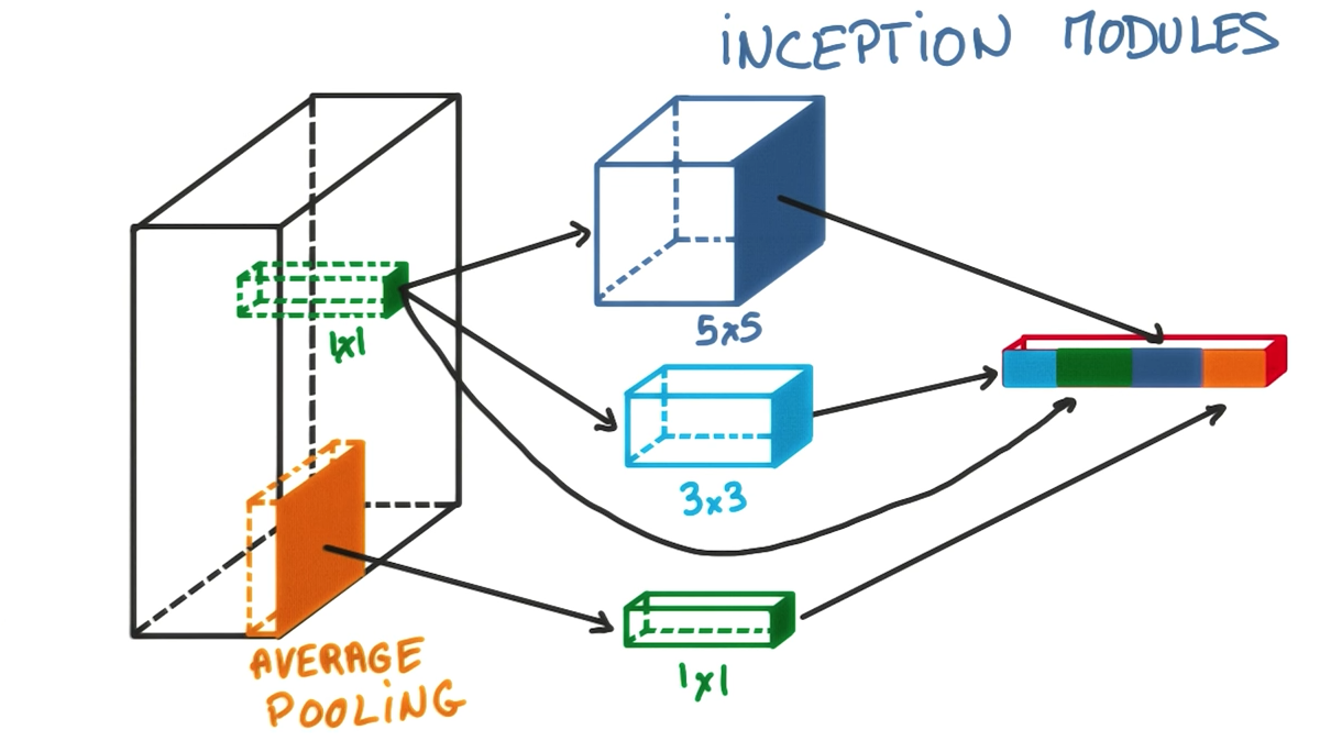
• The main idea behind inception modules is that a 5 x 5 kernel and 3 x 3 kernel followed by a 1 x 1 convolution may both be beneficial to the modelling power of your architecture, so we could just use both, and the model will often perform better than using a single convolution. This video explains the inception module in more detail.

Modelling label noise through probabilistic methods

• The label noise was modelled by first assuming that a true label m is generated from an image s with some conditional probability: \(p(m \vert{} s)\). Usually any form of deep neural networks (and general supervised ML) tries to learn this underlying probability distribution. Several learning algorithms such as binary logistic regression, softmax regression, and linear regression have a probabilistic interpretation of trying to model some underlying distribution. Here are a few examples:

  • Binary logistic regression tries to model a bernoulli distribution by conditioning the label \(y_n\) on the input \(x\) and the weights of the model \(w\): \(p(y_n = 1 \vert{} x_n; w) = h_w(x_n)\) where \(h\) is our model that we learn. More generally, we have the likelihood \(L = \prod h_w(x_n)^{y_n} * (1 - h_w(x_n))^{1-y_n}\). We can then maximize the likelihood (or more typically, minimize the negative log likelihood) by applying gradient descent.
  • Linear regression can be interpretted as the real-valued output, \(y\), being a linear function of the input \(x\) with Gaussin noise \(n_1 \tilde{} N(\mu, \sigma)\) added to it. Then we can write the log likelihood as \(l(\theta) = \sum_i p(y_n \vert{} \theta * x, \sigma^2) = \sum_i \frac{-1}{2\sigma^2}(y_n - \theta^T x)^2 + Nlog(\sigma^2)\).
  • What these probabalistic interpretations let us do is see the assumptions our models make, which is key if we want to simulate the real world. For example, these probability distributions show us that a key assumption is that our data are independent of each other. More specifically for typical linear regression, we also assume that the noise in our model is drawn from a normal distribution with linear mean and constant variance.
• This paper tries to model a similar probability distribution \(p(m \vert{} s)\) but with deep neural networks. It further takes that probabilty distribution of labels and adds a corrupting probability. The ideal label was \(m\) but we observe, in our training set, a noisy label \(\hat{m}\) with probability \(p(\hat{m} \vert{} m)\).
• These probabilities can be drawn from any distribution; the researchers chose an asymmetric binary one. This allows us to account for the fact that even doctors disagree on the true label, so we better model real-world scenarios.

Training the Model

• The training was done with TensorFlow across several different workers and GPUs. The model was pre-initialized with weights learned by the inception-v3 architecture on the ImageNet dataset.
• This method of “transfer learning”, or transferring knowledge from one task to another, has recently gained popularity. The idea is that with learning parameters on ImageNet first, the model learns weights that aid with basic object recognition. Then, the model is trained on a more specific dataset to adjust its later layers, which model higher-level features of what we desire to learn.

Results

• The results support the researcher’s thesis that generalization accuracy improves if the amount of information in the desired outputs is increased.
• Training was done with 5-class loss. Results reported included the 5-class error, binary AUC, and specifity.
• The hyperparameters were tuned with grid search. Methods to avoid overfitting that were used include L1 and L2-regularization as well as dropout throughout the networks. More information about regularization methods to prevent overfitting is in one of my blog posts here.
• The “Weighted Doctor Network” (the network that averages weights of predictions given by several different models, learned for a particular doctor) performed best with a 5-class error fo 20.58%, beating out the baseline inception net and the expectation-maximization algorithm that had 23.83% and 23.74% error respectively.

Grid Search

• Grid search is a common method for tuning the hyperparameters for a deep model. Deep neural networks often require careful hyperparemeter tuning; for example, a learning rate that is too large or one that does not decay as training goes on may cause the algorithm to overshoot the minima and start to diverge. Therefore, we look at all the possible sequences of hyperparameters and pick the one that performs the best.
• Specifically, we enumerate values for our hyperparameters:
  • learning_rates = [0.0001, 0.001, 0.01, 0.1]
  • momentum_consts = [0.1, 0.5, 1.0]
  • dropout_probability = [0.1, 0.5, 0.8]
• Next we do a search over all possible values. To evaluate the performance, it is important to use the validation set or k-fold cross validation. Never touch the test set during training:
  • for lr in learning_rates:
    • for momentum in momentum_consts:
      • for dropout in dropout_probs:
        • model = trained_model(X_train, y_train, lr, momentum, dropout) # calls the function that trains the model
        • cv_error = cross_validate(model, X_train, y_train)
        • update best cv error and hyperparams if less error is found
  • Finally, train a model with the selected hyperparameters.
• As you may have noticed, this method can get expensive as the number of different hyperparameters or different values for each goes up. For \(n\) different parameters with \(k\) possibilies we have to consider \(k^n\) different tuples.

Conclusion

• The paper showed that there are more effective methods to use the noise in labels than using a probability distribution or voting method. The network in this paper seeks to model the labels given by each individual doctor, and learn how to weight them optimially.

Future Application

• This new method of modelling noise in the training datasets is pretty cool. I think it bettter models real-world datasets, where “predictions”, or diagnoses are made by experts with varying levels of experience, biases, and predispositions. For deep learning to advance in the medical field, modelling this aspect of medicine well will be essential. It also has application to other fields where noisy labels exist in any fashion. Here is an example tensorflow implementation of training on corrupted labels.