Optimizing deep neural networks has long followed a general tried-and-true template. Generally, we randomly initialize our weights, which can be thought of as randomly picking a place on the “hill” which is the optimization landscape. There are some tricks we can do to achieve better initialization schemes, such as the He or Xavier initialization.

Then, we follow the gradient and update our parameters until we’ve met some stopping criterion. This is known as gradient descent. More commonly, stochastic gradient descent is used to add noise (via approximating the gradient instead of computing the exact gradient) to the optimization process and speed up training time. Additionally, vanilla SGD is less common now, with practitioners instead opting for methods that add in momentum or adaptive learning rate techniques.

It’s natural to question theoretical - and practical - aspects of this common technique. What guarantees does it provide, and what are some conditions in which it could fail? Here, I’ll attempt to dissect some of these questions so we can better understand what to watch out for when optimizing deep networks.

Precursor: Convexity and the Hessian

Say we want to optimize \(f(x)\) where \(x\) are our parameters that we want to learn. The question of convexity arises. Is \(f\) convex, meaning that any local minimum we achieve is the optimal solution to our problem? Or is \(f\) nonconvex, in which case local minima can be larger than global minima? It turns out that the Hessian, or the matrix of \(f\)’s second derivatives, can tell us a lot about this.

The Hessian is real and symmetric, since in general we assume that the second derivatives exist and \(\frac{dy}{dx_1 x_2} = \frac{dy}{dx_2 x_1}\)for the functions that we are considering (Schwarz’s theorem provides the conditions that need to be true for this to hold). For example, the Hessian for a function \(y = f(x_1, x_2)\) could be expressed as

\[\begin{bmatrix} \frac{dy}{dx_1x_1} & \frac{dy}{dx_1x_2} \\ \frac{dy}{dx_2x_1} & \frac{dy}{dx_2x_2}\end{bmatrix}\]

Real symmetric matrices have nice properties:

• All eigenvalues are real and distinct eigenvalues correspond to distinct eigenvectors
• The eigenvectors of distinct values are orthogonal, and therefore form a basis for \(R^n\), where \(n\) is the dimension of the row/column space of the matrix.
• Thus, the matrix is diagonalizable, i.e. \(Q^{-1} H Q = D\), where \(D\) is a diagonal matrix with the eigenvalues on the diagonal, and \(Q\)’s column vectors form an orthonormal basis for \(R^n\). This is a result of the Spectral Theorem.

Next, a positive definite matrix is a symmetric matrix that has all positive eigenvalues. One way to determine if a function is convex is to check if its Hessian is positive definite.

To show this, it is enough to show that \(z^T H z > 0\) for any real vector \(z\). To see why all positive eigenvalues imply this, first let’s consider the case where \(z\) is an eigenvector of \(H\). Since \(Hz = \lambda z\) we have

\(z^T H z = z^T\lambda z = \lambda z^Tz = \lambda \vert \vert z\vert \vert^2 > 0\) since \(\lambda >0\)

To prove this for an arbitrary vector \(z\), we first note that we can diagonalize \(H\) as follows:

\[z^T H z = z^T Q \Lambda Q^{-1}z\]

Where \(Q\) is a matrix whose columns are (distinct) eigenvectors of \(H\) and \(\Lambda\) is a diagonal matrix with the corresponding eigenvalues on its diagonal. We know that this diagonalization is possible since \(H\) is real and symmetric.

As mentioned, the eigenvectors are orthogonal. Since \(Q\) is a matrix whose columns are the eigenvectors, \(Q\) is an orthogonal matrix, so we have \(Q^{-1} = Q^T\), giving us:

\[z^T Q \Lambda Q^Tz >0\]

Let’s define \(s = Q^T z\), so we now have \(s^T \Lambda s > 0\). Taking

\[s = \begin{bmatrix} s_1 \\ … \\ s_n \end{bmatrix}\]

and

\[\Lambda = \begin{bmatrix} \lambda_1 & 0 &… & 0 \\ 0 & \lambda_2 & … & 0 \\ … & … & … & … \\ 0 & 0 & … & \lambda_n \end{bmatrix}\]

We now have

\[\begin{bmatrix} s_1 & … & s_n \end{bmatrix} \begin{bmatrix} \lambda_1 & 0 &… & 0 \\ 0 & \lambda_2 & … & 0 \\ … & … & … & … \\ 0 & 0 & … & \lambda_n \end{bmatrix} \begin{bmatrix} s_1 \\ … \\ s_n \end{bmatrix} = \begin{bmatrix} s_1 & … & s_n \end{bmatrix} \begin{bmatrix} \lambda_1 s_1 \\ … \\ \lambda_ns_n \end{bmatrix} = \sum_{i=1}^{N}\lambda_is_i^2 > 0\]

Which is true since all the eigenvalues are positive.

As an example of using this analysis to prove the convexity of a machine learning problem, we can take the loss function of the (l2-regularized) SVM:

\[L(w) = \lambda \sum_n w_n^2 + \sum_n \max (0, 1 - y_n(w^Tx_n))\]

The derivatives for each \(w_m\) are \(\frac{dL}{dw_m} = \lambda w_m + \sum \textbf{1} (y_n w^T x_n < 1)(-y_nx_{nm})\), where \(\textbf{1}\) denotes the indicator function that returns the second argument if its first argument is true, and \(x_{nm}\) denotes the \(m\)th feature of the \(n\)th feature vector.

The second derivatives can be characterized as \(\frac{dL}{dw_m w_k}, k != m\) and \(\frac{dL}{dw_m^2}\). The latter derivatives will appear as the diagonal entries of the Hessian.

For the first case, since our expression \(\frac{dL}{dw_m}\) is constant with respect to \(w_k\) the derivative is simply \(0\). For the second case, the derivative is simply \(\lambda\). Therefore, our Hessian is the following diagonal matrix:

\[\begin{bmatrix} \lambda & 0 &… & 0 \\ 0 & \lambda & … & 0 \\ … & … & … & … \\ 0 & 0 & … & \lambda \end{bmatrix}\]

Since this is a diagonal matrix, the eigenvalues are simply the entries on the diagonal. Since the regularization constant \(\lambda > 0\), the Hessian is positive definite, therefore the above formulation of the hinge loss is a convex problem. We could have alternatively shown that \(z^T H z > 0\) as well, since \(H z\) simply scales \(z\) by a positive scalar.

Ok…But what about Neural Networks?

The optimization problem for neural networks are generally highly nonconvex, making optimizing deep neural networks much tougher. Fortunately, there are still some applications of the Hessian that we could use.

Local Minima

First, it may be worth it to know if we are at a local minimum at any point during our optimization process. In some cases, if this occurs early in our training process or at a high value for our objective function, then we could consider restarting our training/initialization process or randomly update our objective to “kick” our parameters out of the bad local minima.

Even though the Hessian may not be positive definite at any given point, we can check if we’re at a local minimum by examining the Hessian. This is basically the second derivative test in single-variable calculus. Consider the Taylor Series expansion of our objective \(f\) around \(x_0\):

\[f(x)\approx f(x_0) + (x-x_0)\nabla_xf(x_0) + \frac{1}{2}(x-x_0)^T\textbf{H}(x-x_0)\]

If we’re at a critical point, it is a potential local minimum and we have \(\nabla_x f(x) = 0\). Considering an SGD update \(x = x_0 - \epsilon u\), we have

\[f(x_0-\epsilon u) \approx f(x_0) + \frac{1}{2}(x_0 - \epsilon u - x_0)^T\textbf{H}(x_0 - \epsilon u - x_0)\] \[f(x_0-\epsilon u) \approx f(x_0) + \frac{1}{2}\epsilon^2 u^T\textbf{H} u\]

If the Hessian is positive definite at \(x_0\), then it tells us that any direction \(u\) in which we choose to travel will result an increased value of the objective function (since the term \(\frac{1}{2}\epsilon^2 u^T\textbf{H} u > 0\)), so we are at a local minimum. We can similarly use the idea of negative definiteness to see if we are at a local maximum.

Are local minima really that big of a problem?

Arguably, the goal of fitting deep neural networks may not be to reach the global minimum, as this could result in overfitting, but rather find an acceptable local minima that obains good performance on the test set. In this paper, the authors state that “while local minima are numerous, they are relatively easy to find, and they are all more or less equivalent in terms of performance on the test set”. In the Deep Learning Book, Goodfellow et al. state the early convergence to a high value for the objective is generally not due to local minima, and this can be verified by plotting the norm of the gradient throughout the training process. The gradient at these supposed local minima exhibit healthy norms, indicating that the point is not actually a local minima.

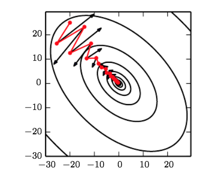
A Poorly Conditioned Hessian

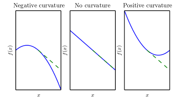
There are some cases where the regular optimization process - a small step in the direction of the gradient - could actually fail, and increase the value of our objective function - couteractive to our goal. This happens due to the curvature of the local region of our objective function, and can be investigated with the Hessian as well.

How much will a gradient descent update change the value of our objective? First, let’s again look at the Taylor series expansion for an update \(x \leftarrow x_0 - \epsilon \textbf{g}\) where \(\textbf{g} = \nabla f(x_0)\):

\[f(x_0 - \epsilon\textbf{g})\approx f(x_0) + (x_0 - \epsilon \textbf{g}-x_0)\textbf{g} + \frac{1}{2}(x_0 - \epsilon \textbf{g}-x_0)^T\textbf{H}(x_0 - \epsilon \textbf{g}-x_0)\] \[f(x_0 - \epsilon\textbf{g})\approx f(x_0) -\epsilon\textbf{g}^T\textbf{g} + \frac{1}{2}\epsilon^2\textbf{g}^T\textbf{H}\textbf{g}\]

We can see that the decrease in the objective is related to 2nd order information, specifically the term \(g^T H g\). If this term is negative, then the decrease in our objective is greater than our (scaled) squared gradient norm, if it is positive, then the decrease is less, if it is zero, the decrease is completely given by first-order information.

“Poor Conditioning” refers to the Hessian at the point \(x_0\) being such that it results in an increased value of our objective function. This can happen if the term that indicates our decrease in our objective is actually greater than \(0\):

\(-\epsilon g^Tg + \frac{1}{2}\epsilon^2g^T Hg > 0\) which corresponds to \(\epsilon g^T g < \frac{1}{2}\epsilon^2g^THg\)

This can happen if the Hessian is very large, in which case we’d want to use a smaller learning rate than \(\epsilon\) to offset some of the influence of the curvature. An intuitive justification for this is that due to the large magnitude of curvature, we’re more “unsure” of our gradient updates, so we want to take a smaller step, and therefore have a smaller learning rate.

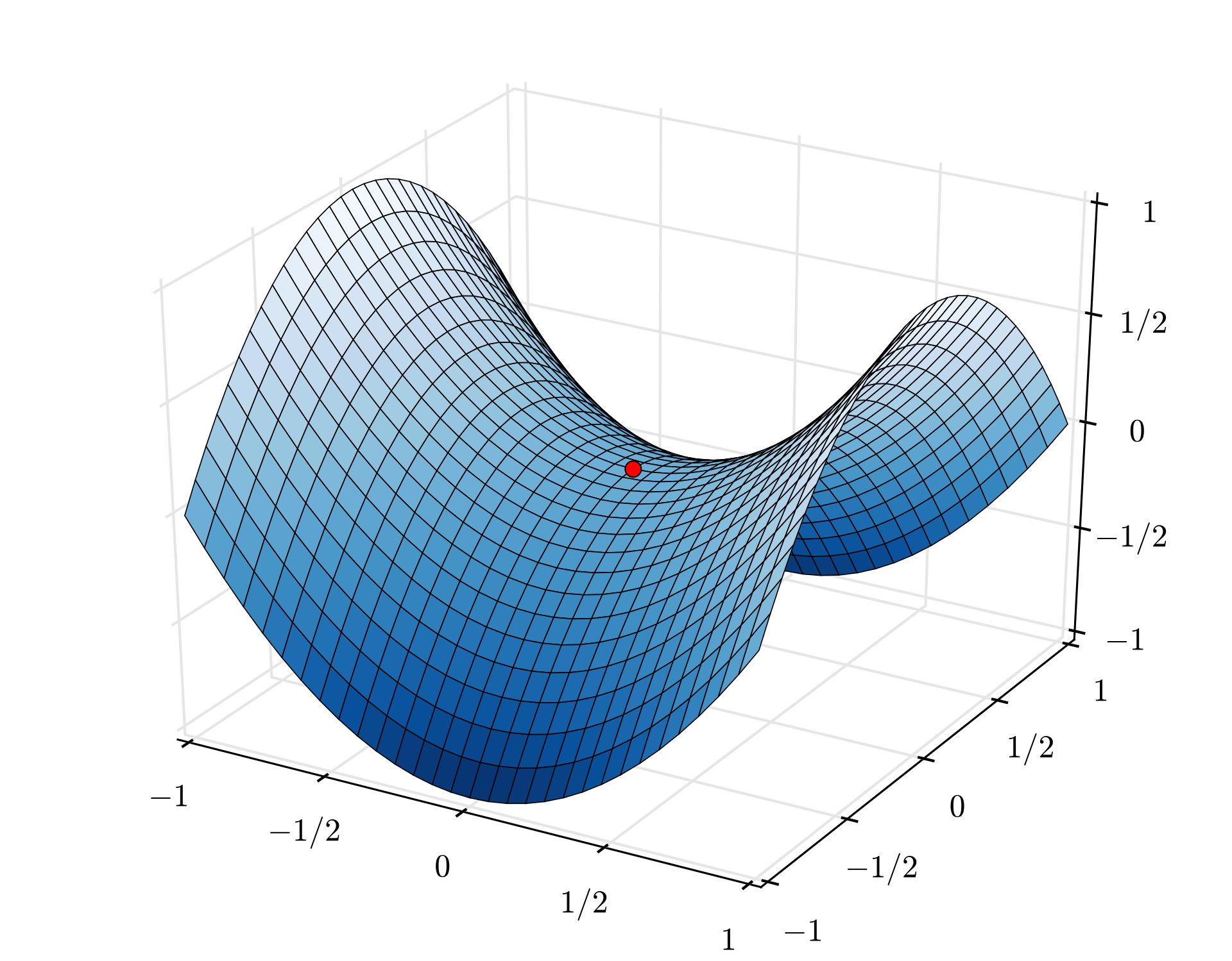
Saddle Points

Getting stuck at a saddle point is a very real issue for optimizing deep neural networks, and arguably a more important issue than getting stuck at a local minima (see http://www.offconvex.org/2016/03/22/saddlepoints/). One explanation of this is that it’s much more likely to arrive at a saddle point than a local minimum or maximum: the probability of a given point in an \(n\) dimensional optimization space being a local minimum or maximum is just \(\frac{1}{2^n}\).

A saddle point is defined as a point with \(0\) gradient, but the Hessian is neither positive definite or negative definite. It is possible that learning would stop if we are relying only on first-order information (i.e. since \(\nabla_x f(x) = 0\), the weights will not be updated) but in practice, using techniques such as momentum reduce the chance of this.

Around a saddle point, the expansion of our objective is similar to the expansion at a local minimum:

\[f(x_0-\epsilon u) \approx f(x_0) + \frac{1}{2}\epsilon^2 u^T\textbf{H} u\]

Here, \(\textbf{H}\) is not positive definite, so we may be able to pick certain directions \(u\) that increase or decrease the value of our objective. Concretely, if we pick \(u\) such that \(u^T \textbf{H}u < 0\), then \(u\) is a direction that would decrease the value of our objective (since the term \(\frac{1}{2}\epsilon^2 u^T\textbf{H} u < 0\) decreases the value of our objective) , and we can update our parameters with \(u\). Ideally we’d like to find a \(u\) such that \(u^T\textbf{H}u\) is significantly less than \(0\), so that we have a steeper direction of descent to travel in.

How do we know what functions have saddle points that are “well-behaved” like this? Ge et al. in their paper introduced the notion of “strict saddle” functions. One of the properties of these “strict saddle” functions is that at all saddle points \(x\), the Hessian has a (significant) negative eigenvalue, which means that we can pick the eigenvector corresponding to this eigenvalue as our direction to travel in if we are at a saddle point.

However, it is often infeasible to compute the Hessian while training deep learning models, since it is computationally expensive. How can we escape saddle points using only first-order information?

Get et al. in their paper also describe a variant of stochastic gradient descent which they call “noisy stochastic gradient descent”. The only variant is that some random noise is added to the gradient:

\[\textbf{g} = \nabla_\theta \frac{1}{m}\sum_{i=1}^{m} L(f(x^i; \theta), y^i)\] \[\theta_{t+1} \leftarrow{} \theta_{t} - \epsilon (\textbf{g} + \nu)\]

where \(\nu\) is random noise sampled from the unit sphere. This ensures that there is noise in every direction, allowing this variant of SGD to explore the region around the saddle point. The authors show that this noise can help escape from saddle points for strict-saddle functions.

The authors mention in the corresponding blog post that it is useful to think of a saddle point as unstable, so slight perturbations can be effective in order to kick your weights out of the saddle point. To me this indicates that any perturbation in addition to the regular SGD update could be beneficial to continue optimization at a saddle point, so techniques such as momentum would be helpful as well.

Computing the Hessian

Most of these methods discussed involve the need to compute the Hessian, which is often unrealistic in practice due to the aformented reasons. However, we can use finite difference methods in order to approximate the Hessian, which may be enough to do our job. To understand this, first we can consider the limit definition of the derivative in the single-variable case:

\[\frac{d}{dx} f(x) = \lim_{h \rightarrow{} 0} \frac{f(x + h) - f(x)}{h}\]

This means an approximation for \(\frac{d}{dx}f(x)\) can be given by

\[\frac{f(x + h) - f(x)}{h}\]

where our approximation improves with a smaller \(h\) but we run into numerical stability issues if we take \(h\) to be too small. It turns out that a slightly better approximation would be to use the centered version of the above (see the explanation on CS 231n for details):

\[\frac{d}{dx}f(x) \approx \frac{f(x + h) - f(x-h)}{2h}\]

For vector-valued functions, we can generalize this idea to several dimensions:

\[\frac{d}{dx_i}f(x) \approx \frac{f(x + h s_i) - f(x - h s_i)}{2h}\]

where \(s_i\) is a vector that has \(1\) as its \(i\)th entry, and is zero everywhere else. We’re basically taking the unit vector pointing in that direction, scaling it so that it is small, and adding that to our setting of parameters given by the vector \(x\).

It turns out that this identity can be further generalized, to approximate the gradient-vector product (i.e. the product of the gradient times a given vector). We simply remove the constraint that \(s_i\) is the unit vector pointing in a particular direction, and instead let it be any vector \(u\). This lets us approximate the gradient vector product:

\[\nabla_x f(x)^T u \approx \frac{f(x + h u) - f(x - h u)}{2h}\]

It’s quite simple to extend this to computing the Hessian-vector product: given the gradient, the gradient of the gradient is the Hessian. This means that we can replace the gradient on the left hand side of the above equation with the Hessian, and the function on the right hand side with the gradient:

\[H u \approx \frac{\nabla_xf(x + h u) - \nabla_xf(x - h u)}{2h}\]

which gives us the Hessian-vector product.

Takeaways

The Hessian can give us useful second order information when optimizing machine learning algorithms, though it is computationally tough to compute in practice. By analyzing the Hessian, we may be able to get information regarding the convex nature of our problem, and it can also help us determine local minima or “debug” gradient descent when it actually fails to reduce our cost function or gets stuck at a saddle point.

Sources

1. Escaping from Saddle Points
2. Paper: Escaping from Saddle Points - Online SGD for Tensor Decomposition
3. Deep Learning Book Ch. 8
4. Explanation of approximating gradient-vector products

Notes

[4/7/19] - Added further explanation for the claim that “The eigenvectors of distinct values are orthogonal, and therefore form a basis for \(R^n\)”

[4/7/19] - Added a note about the indicator function notation that I used when explaining the L2-regularized SVM.

[5/7/19] - Fixed an incorrect equation and added some clarifications.

[5/30/19] - Fixed the gradient in the SVM example.

[6/7/19] - Added a note about the Spectral Theorem.