Introduction/Background

In machine learning, we often start off by writing down a probabalistic model that defines our data. We then go on to write down a likelihood or some type of loss function, which we then optimize over to get the optimal settings for the parameters that we seek to estimate. Along the way, techniques such as regularization, hyperparameter tuning, and cross-validation can be used to ensure that we don’t overfit on our training dataset and our model generalizes well to unseen data.

Specifically, we have a few key functions and variables: the underlying probability distribution \(p(x, y)\) which generate our training examples (pairs of features and labels), a training set \((x, y)_{i = 1}^{D}\) of \(D\) examples which we observe, and a model \(h(x) : x \rightarrow{} y\) which we wish to learn in order to produce a mapping from \(x\) to \(y\). This function \(h\) is selected from a larger function space \(H\).

For example, if we are in the context of linear regression models, then all functions in the function space of \(H\) will take on the form \(y_i = x_{i}^T \beta\) where a particular setting of our parameters \(\beta\) will result in a particular \(h(x)\). We also have some function \(L(h(x), y)\) that takes in our predictions and labels, and quantifies how accurate our model is across some data.

Ideally, we’d like to minimize the risk function

\[R[h(x)] = \sum_{(x, y)} L( h(x), y) p(x, y)\]

across all possible \((x, y)\) pairs. However, this is impossible since we don’t know the underlying probability distribution that describes our dataset, so instead we seek to approximate the risk function by minimizing a loss function across the data that we have observed:

\[\frac{1}{N} \sum_{i = 1}^{N} L(h(x), y)\]

Linear Models

If we assume that our data are roughly linear, then we can write a relationship between our features and real-valued outputs: \(y_i = x_i^T \beta + \epsilon\) where \(\epsilon \tilde{} N(0, \sigma^2)\). This essentially means that our data has a linear relationship that is corrupted by random Gaussian noise that has zero mean and constant variance.

This has the implication that \(y_i\) is a Gaussian random variable, and we can compute its expectation and variance:

\[E[y_i] = E[x_i^T \beta + \epsilon] = x_i^T \beta\] \[Var[y_i] = Var[x_i^T \beta + \epsilon] = \sigma^2\]

We can now write down the probability of observing a value \(y_i\) given a certain set of features \(x\):

\[p(y_i | x_i) = N(y_i | x_i^T \beta, \sigma^2)\]

Next, we can write down the probability of observing the entire dataset of \((x, y)\) pairs. This is known as the likelihood, and it’s simply the product of observing each of the individual feature, label pairs:

\[L(x,y) = \prod_{i = 1}^{n} N(y_i | x_i \beta, \sigma^2)\]

As a note, writing down the likelihood this way does assume that our training data are independent and identically distributed, meaning that we are assuming that each of the training samples have the same probability distribution, and are mutually independent.

If we want to find the \(\hat{\beta}\) that maximizes the chance of us observing the training examples that we observed, then it makes sense to maximize the above likelihood. This is known as maximum likelihood estimation, and is a common approach to many machine learning problems such as linear and logistic regression.

In other words, we want to find

\[\hat{\beta} = argmax_{\beta} \prod_{i = 1}^{n} N(y_i | x_i \beta, \sigma^2)\]

To simplify this a little bit, we can write out the normal distribution, and also take the log of the function, since the \(\hat{\beta}\) that maximizes \(L\) will also maximize \(log(L)\). We end up with

\[\hat{\beta} = argmax_{\beta} log \prod_{i = 1}^{n} \frac{1}{\sqrt(2 \pi \sigma^2}e^-\frac{(y_i - x_i \beta)^2}{2 \sigma^2}\]

Distributing the log and dropping constants (since they don’t affect the value of our parameter which maximizes the expression), we obtain

\[\hat{\beta} = argmax_{\beta} \sum_{i = 1}^{N} -(y_i - x_i \beta)^2\]

Since minimizing the opposite of a function is the same as maximizing it, we can turn the above into a minimization problem:

\[\hat{\beta} = argmin_{\beta} \sum_{i = 1}^{N} (y_i - x_i \beta)^2\]

This is the familiar least squares estimator, which says that the optimal parameter is the one that minimizes the \(L2\) squared norm between the predictions and actual values. We can use gradient descent with some initial setting of \(\beta\) and be guaranteed to get to a global minimum (since the function is convex) or we can explicitly solve for \(\beta\) and obtain the same answer.

Right now is a good time to think about the assumptions of this linear regression model. Like many models, it assumes that the data are drawn independently from the same data generating distribution. Furthermore, it assumes that this distribution is normal with a linear mean and constant variance. It also has a more implicit assumption: that the parameter \(\beta\) which we wish to estimate is not a random variable itself, and we will show how relaxing this assumption leads to a regularized linear model.

Regularization

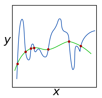
Regularization is a popular approach to reducing a model’s predisposition to overfit on the training data and thus hopefully increasing the generalization ability of the model. Previously, we sought to learn the optimial \(h(x)\) from the space of functions \(H\). However, if the whole function space can be explored, and our samples were observed with some amount of noise, then the model will likely select a function that overfits on the observed data. One way we can combat this is by limiting our search to a subspace within \(H\), and this is exactly what regularization does.

To regularize a model, we take our loss function and add a regularizer to it. Regularizers take the form \(\lambda R(\beta)\) where \(R(\beta)\) is some function of our parameters, and \(\lambda\) is a hyperparameter describing our regularization constant. Using this rule, we can write out a regularized version of our loss function above, giving us a model known as ridge regression:

\[\hat{\beta} = argmin_{\beta} \sum_{i = 1}^{N} (y_i - x_i \beta)^2 + \lambda \sum_{i = 1}^{j} \beta_j^2\]

What’s interesting about regularization is that it can be more deeply understood if we reconsider our original probabalistic model. In our original model, we conditioned our outputs on a linear function of the parameter which we wish to learn \(\beta\). Instead of considering \(\beta\) as a fixed quantity that we want a point estimate of, we can consider \(\beta\) itself as a random variable drawn from a certain probability distribution. This is known as the prior probability distribution, because we assign \(\beta\) some probability without having observed the associated \((x, y)\) pairs. Imposing a prior would be especially useful if we had some information about the parameter before observing any of the training data (possibly from domain knowledge), but it turns out that imposing a Gaussian prior even in the absence of actual prior knowledge leads to interesting properties (see the Deep Learning Book chapter on regularization for more details about this). In particular, we can condition \(\beta\) as on a Gaussian with 0 mean and constant variance [1]:

\[\beta \tilde{} N(0, \lambda^{-1})\]

As a consequence, we must adjust our probability of observing a particular \((x, y)\) pair to accommodate the probability of observing the parameter that generated this pair. We obtain a new expression for our likelihood:

\[L(x,y) = \prod_{i = 1}^{n} N(y_i | x_i \beta, \sigma^2) N(\beta | 0, \lambda^{-1})\]

Similar to the previously discussed method of maximum likelihood estimation, we can estimate the parameter \(\beta\) to be the \(\hat{\beta}\) that maximizes the above function:

\[\hat{\beta} = argmax_{\beta} \sum_{i = 1}^{N} log N(y_i | x_i \beta, \sigma^2) + log N(\beta | 0, \lambda^{-1})\]

This is the maximum a posteriori estimate of \(\beta\), and it only differs from the maximum likelihood estimate in that the former takes into account previous information, or a prior distribution, on the parameter \(\beta\). In fact, the maximum likelihood estimate of the parameter can be seen as a special case of the maximum a posteriori estimate, where we take the prior probability distribution on the parameter to just be a constant.

Since (dropping unneeded constants) \(N(\beta, 0, \lambda^{-1}) = exp(\frac{- \beta^{2}}{2 \lambda^{-1}})\), after taking the log, and minimizing the negative of the above function we obtain the familiar regularizer \(\frac{1}{2} \lambda \beta^2\) and our squared loss function \(\sum_{i = 1}^{N} (y_i - x_i \beta)^2\) is the same as the loss function we obtained without regularization. In this way, \(L2\) regularization on a linear model can be thought of as imposing a Bayesian prior on the underlying parameters which we wish to estimate.

Aside: interpreting regularization in the context of bias and variance

The error of a statistical model can be decomposed into three distinct sources of error: error due to bias, error due to variance, and irreducible error. They are related as follows:

\[Err(x) = bias(X)^2 + var(x) + \epsilon\]

Given a constant error, this means that there will always be a tradeoff between bias and variance. Having too much bias or too much variance isn’t good for a model, but for different reasons. A high bias, low variance model will likely end up being inaccurate across both the training and testing datasets, and its predictions will likely not deviate too much based on the data sample it is trained on. On the other hand, a low-bias, high-variance model will likely give good results on a training dataset, but fail to generalize as well on a testing dataset.

The Gauss-Markov theorem states that in a linear regression problem, the least squares estimator has the lowest variance out of all other unbiased estimators. However, if we consider biased estimators such as the estimator given by ridge regression, we can arrive at a lower variance, higher-bias solution. In particular, the expectation of the ridge estimator (derived here) is given by:

\[\beta - \lambda (X^TX + \lambda I)^{-1} \beta\]

The bias of an estimator is defined as the difference between the parameter’s expected value and the true parameter \(\beta\): \(bias(\hat{\beta}) = E[\hat{\beta}] - \beta\)

As you can see, the bias is proportional to \(\lambda\) and \(\lambda = 0\) gives us the unbiased least squares estimator since \(E[\hat{\beta}] = \beta\). Therefore, assuming a constant total error for the least squares estimator and the ridge estimator, the variance for the ridge estimator is lower. A more complete discussion, including formal calculations for the bias and variance of the ridge estimator compared to the least squares estimator, is given here.

A linear algebra perspective

To see why regularization makes sense from a linear algebra perspective, we can write down our least squares estimate in vectorized form:

\[argmin_{\beta} { (y - X\beta)^T (y - X \beta) }\]

Next, we can expand this and simplify a little bit:

\[argmin_{\beta} (y^T - \beta^TX^T)(y - X\beta)\] \[= argmin_{\beta} -2y^TX\beta + \beta^TX^TX\beta\]

where we have dropped the terms that are not a factor of \(\beta\) since they will zero out when we differentiate.

To minimize, we differentiate with respect to \(\beta\):

\[\frac{\delta L}{\delta \beta} = -2 y^TX + 2X^TX\beta\]

Setting the derivative equal to zero gives us the closed form solution of \(\beta\) which is the least-squares estimate [2]:

\[\hat{\beta} = (X^TX)^{-1} y^TX\]

As we can see, in order to actually compute this quantity the matrix \(X^T X\) must be invertible. The matrix \(X^T X\) being invertible corresponds exactly to showing that the matrix is positive definite, which means that the scalar quantity \(z^T X^T X z > 0\) for any real, non-zero vectors \(z\). However, the best we can do is show that \(X^T X\) is positive semidefinite.

To show that \(X^TX\) is positive semidefinite, we must show that the quantity \(z^T X^T X z \geq 0\) for any real, non-zero vectors \(z\).

If we expand out the quantity \(X^T X\), we obtain \(\sum_{i = 1}^{N} x_i x_i^T\) and it follows that the quantity \(z^T (\sum_{i = 1}^{N} x_i x_i^T) z = \sum_{i = 1}^{N} (x_i^Tz)^2 \geq 0\). This means that in sitautions where this quantity is exactly \(0\), the matrix \(X^T X\) cannot be inverted and a closed-form least squares solution cannot be computed.

On the other hand, expanding out our ridge estimate which has an extra regulariztion term \(\lambda \sum_{i} \beta_i^2\), we obtain the derivative

\[\frac{\delta L}{\delta \beta} = -2 y^TX + 2X^TX\beta + 2 \lambda \beta\]

Setting this quantity equal to zero, and rewriting \(\lambda \beta\) as \(\lambda I \beta\) (using the property of multiplication with the identity matrix), we now obtain

\[\beta (X^TX + \lambda I) = y^T X\]

giving us the ridge estimate

\[\hat{\beta_{ridge}} = (X^TX + \lambda I)^{-1} y^TX\]

The only difference in this closed-form solution is the addition of the \(\lambda I\) term to the quantity that gets inverted, so we are now sure that this quantity is positive definite if \(\lambda > 0\). In other words, even when the matrix \(X^T X\) is not invertible, we can still compute a ridge estimate from our data [3].

Regularizers in neural networks

While techniques such as L2 regularization can be used while training a neural network, employing techniques such as dropout, which randomly discards some proportion of the activations at a per-layer level during training, have been shown to be much more successful. There is also a different type of regularizer that takes into account the idea that a neural network should have sparse activations for any particular input. There are several theoretical reeasons for why sparsity is important, a topic covered very well by Glorot et al. in a 2011 paper.

Since sparsity is important in neural networks, we can introduce a constraint that can gaurantee us some degree of sparsity. Specifically, we can constrain the average activation of a particular neuron in a particular hidden layer.

In particular, the average activation of a neuron in a particular layer, weighted by the input into the neuron, can be given by summing over all of the activation - input pairs: \(\hat{\rho} = \frac{1}{m} \sum_{i = 1}^{N} x_i a_i^2\). Next, we can choose a hyperparameter \(\rho\) for this particular neuron, which represents the average activation we want it to have - for example, if we wanted this neuron to activate sparsely, we might set \(\rho = 0.05\). In order to ensure that our model learns neurons which sparsely activate, we must incorporate some function of \(\hat{\rho}\) and \(\rho\) into our cost function.

One way to do this is with the KL divergence, which computes how much one probability distribution (in this case, our current average activation \(\hat\rho\)) and another expected probability distribution (\(\rho\)) diverge from each other. If we minimize the KL divergence for each of our neuron’s activations then our model will learn sparse activations. The cost function may be:

\[J_{sparse} (W, b) = J(W, b) + \lambda \sum_{i = 1}^{M} KL(\rho_i || \hat{\rho_i})\]

where \(J(W, b)\) is a regular cost function used in neural networks, such as the cross-entropy loss. The hyperparameter \(\lambda\) indicates how important sparsity is to us - as \(\lambda \rightarrow{} \infty\), we disregard the actual loss function and only aim to learn a sparse representation, and as \(\lambda \rightarrow{} 0\) we disregard the importance of sparse activations and only minimize the original loss function. Additional details on this type of regularization with application to sparse autoencoders are given here.

Recap

As we have seen, regularization can be interpreted in several different ways, each of which gives us additional insight into what exactly regularization accomplishes. A few of the different interpretations are:

1) As a Bayesian prior on the paramaters which we are trying to learn.

2) As a term added to the loss function of our model which penalizes some function of our parameters, thereby introducing a tradeoff between minimizing the original loss function and ensuring our weights do not deviate too much from what we want them to be.

3) As a constraint on the model which we are trying to learn. This means we can take the original optimization problem and frame it in a constrained fashion, thereby ensuring that the magnitude of our weights never exceed a certain threshold (in the case of \(L2\) regularization).

4) As a method of reducing the function search space \(H\) to a new function search space \(H'\) that is smaller than \(H\). Without regularization, we may search for our optimal function \(h\) in a much larger space, and constraining this to a smaller subspace can lead us to select models with better generalization ability.

Overall, regularization is a useful technique that is often employed to reduce the overall variance of a model, thereby improving its generalization capability. Of course, there’s tradeoffs in using regularization, most notably having to tune the hyperparameter \(\lambda\) which can be costly in terms of computational time. Thanks for reading!

Sources

1. Boston University Linear Models Course by Cedric Ginestet

2. Autoencoders and Sparsity, Stanford UFDL

3. Explanation of MAP Estimation

Notes

[1] Imposing different prior distributions on the parameter leads to different types of regularization. A normal distribution with zero mean and constant variance leads to \(L2\) regularization, while a Laplacean prior would lead to \(L1\) regularization.

[2] Technically, we’ve only shown that the \(\hat{\beta}\) we’ve found is a local optimum. We actually want to verify that this is indeed a global minimum, which can be done by showing that the function we are minimizing is convex.

[3] For completeness, it is worth mentioning that there are other solutions if the inverse of the matrix \(X^T X\) does not exist. One common workaround is to use the Moore-Penrose Psuedoinverse which can be computed using the singular value decompisition of the matrix being psuedo-inverted. This is commonly used in implementations of PCA algorithms.

[7/15/19] - Added a note abou the underlying parameters of a model coming from a prior probability distribution.