Introduction

The Word2Vec model has become a standard method for representing words as dense vectors. This is typically done as a preprocessing step, after which the learned vectors are fed into a discriminative model (typically an RNN) to generate predictions such as movie review sentiment, do machine translation, or even generate text, character by character.

Previous Language Models

Previously, the bag of words model was commonly used to represent words and sentences as numerical vectors, which could then be fed into a classifier (for example Naive Bayes) to produce output predictions. Given a vocabulary of \(V\) words and a document of \(N\) words, a \(V\)-dimensional vector would be created to represent the document, where index \(i\) in the vector denotes the number of times the \(i\)th word in the vocabulary occured in the document.

This model represented words as atomic units, assuming that all words were independent of each other. It had success in several fields such as document classification, spam detection, and even sentiment analysis, but its assumptions (that words are completely independent of each other) were too strong for more powerful and accurate models. A model that aimed to reduce some of the strong assumptions of the traditional bag of words model was the n-gram model.

N-gram models and Markov Chains

Language models seek to predict the probability of observing the \(t + 1\)th word \(w_{t + 1}\) given the previous \(t\) words:

\[p(w_{t + 1} | w_1, w_2, ... w_t)\]

Using the chain rule of probabilty, we can compute the probabilty of observing an entire sentence:

\[p(w_1, w_2, ... w_t) = p(w_1)p(w_2 | w_1)...p(w_t | w_{t -1}, ... w_1)\]

Computing these probabilities have many applications, for example in speech recognition, spelling corrections, and automatic sentence completion. However, estimating these probabilites can be tough. We can use the maximum likelihood estimate:

\[p(x_{t + 1} | x_1, ... x_t) = \frac{count(x_1, x_2, ... x_t, x_{t + 1})}{count(x_1, x_2, ... x_t)}\]

However, computing this is quite unrealistic - we will generally not observe enough data from a corpus to obtain realistic counts for any sequence of \(t\) words for any nontrivial value of \(t\), so we instead invoke the Markov assumption. The Markov assumption assumes that the probability of observing a word at a given time is only dependent on the word observed in the previous time step:

\[p(x_{t + 1} | x_1, x_2, ... x_t) = p(x_{t + 1} | x_t)\]

Therefore, the probabilty of a sentence can be given by

\[p(w_1, w_2, ... w_t) = p(w_1)\prod_{i = 2}^{t} p(w_i | w_{i - 1})\]

The Markov assumption can be extended to condition the probability of the \(t\)th word on the previous two, three, four, and so on words. This is where the name of the n-gram model comes in - \(n\) is the number of previous timesteps we condition the current timestep on. The unigram and bigram models, respectively, are given below.

\[p(x_{t + 1} | x_{1}, x_{2}, ... x_{t}) = p(x_{t + 1})\] \[p(x_{t + 1} | x_{1}, x_{2}, ... x_{t}) = p(x_{t + 1} | x_{t})\]

There is a lot more to the n-gram model such as linear interpolation and smoothing techniques, which these slides explain very well. One thing to keep in mind is that as we increase \(n\), the probabilities become more challening to compute, though a smaller \(n\) may make our model less expressive, since aren’t able to learn longer-term conditionings.

The Skip-Gram and Continuous Bag of Words Models

Word vectors, or word embeddings, or distributed representation of words, generally refer to a dense vector representation of a word, as compared to a sparse (ie one-hot) traditional representation. There are actually two different implementations of models that learn dense representation of words: the Skip-Gram model and the Continuous Bag of Words model. Both of these models learn dense vector representation of words, based on the words that surround them (ie, their context).

The difference is that the skip-gram model predicts context (surrounding) words given the current word, wheras the continuous bag of words model predicts the current word based on several surrounding words.

This notion of “surrounding” words is best described by considering a center (or current) word and a window of words around it. For example, if we consider the sentence “The quick brown fox jumped over the lazy dog”, and a window size of 2, we’d have the following pairs for the skip-gram model:

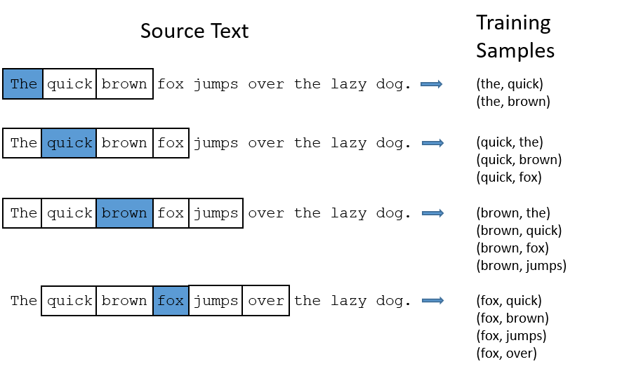
Figure 1: Training Samples (Source, from Chris McCormick’s insightful post)

In contrast, for the CBOW model, we’ll input the context words within the window (such as “the”, “brown”, “fox”) and aim to predict the target word “quick” (simply reversing the input to prediction pipeline from the skip-gram model).

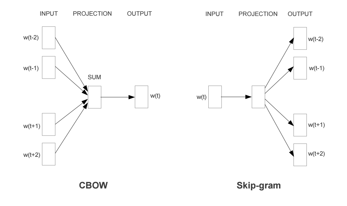
The following is a visualization of the skip-gram and CBOW models:

Figure 2: CBOW vs Skip-gram models. (Source)

In this paper, the overall recommendation was to use the skip-gram model, since it had been shown to perform better on analogy-related tasks than the CBOW model. Overall, if you understand one model, it is pretty easy to understand the other: just reverse the inputs and predictions. Since both papers focused on the skip-gram model, this post will do the same.

Learning with the Skip-Gram Model

Our goal is to find word representations that are useful for predicting the surrounding words given a current word. In particular, we wish to maximize the average log probability across our entire corpus:

\[argmax_{\theta} \frac{1}{T} \sum_{t=1}^{T} \sum_{j \in c, j != 0} log p(w_{t + j} | w_{t} ; \theta)\]

This equation essentially says that there is some probability \(p\) of observing a particular word that’s within a window of size \(c\) of the current word \(w_t\). This probability is conditioned on the current word (\(w_t\)) and some setting of parameters \(\theta\) (determined by our model). We wish to set these parameters \(\theta\) so that this probability is maximized across our entire corpus.

Basic Parametrization: Softmax Model

The basic skip-gram model defines the probability \(p\) through the softmax function. If we consider \(w_i\) to be a one-hot encoded vector with dimension \(N\) and \(\theta\) to be a \(N * K\) matrix embedding matrix (here, we have \(N\) words in our vocabulary and our learned embeddings have dimension \(K\)), then we can define

\[p(w_{i} | w_{t} ; \theta) = \frac{exp(\theta w_i)}{\sum_t exp(\theta w_t)}\]

It is worth noting that after learning, the matrix \(\theta\) can be thought of as an embedding lookup matrix. If you have a word that is represented with the \(k\)th index of a vector being hot, then the learning embedding for that word will be the \(k\)th column. This parametrization has a major disadvantage that limits its usefulness in cases of very large corpuses. Specifically, we notice that in order to compute a single forward pass of our model, we must sum across the entire corpus vocabulary in order to evaluate the softmax function. This is prohibitively expensive on large datasets, so we look to alternate approximations of this model for the sake of computational efficiency.

Hierarchical Softmax

As discussed, the traditional softmax approach can become prohibitively expensive on large corpora, and the hierarchical softmax is a common alternative approach that approximates the softmax computation, but has logarithmic time complexity in the number of words in the vocabulary, as opposed to linear time complexity.

This is done by representing the softmax layer as a binary tree where the words are leaf nodes of the tree, and the probabilities are computed by a walk from the root of the binary tree to the particular leaf. An example of the binary tree of the hierarchical layer is given below:

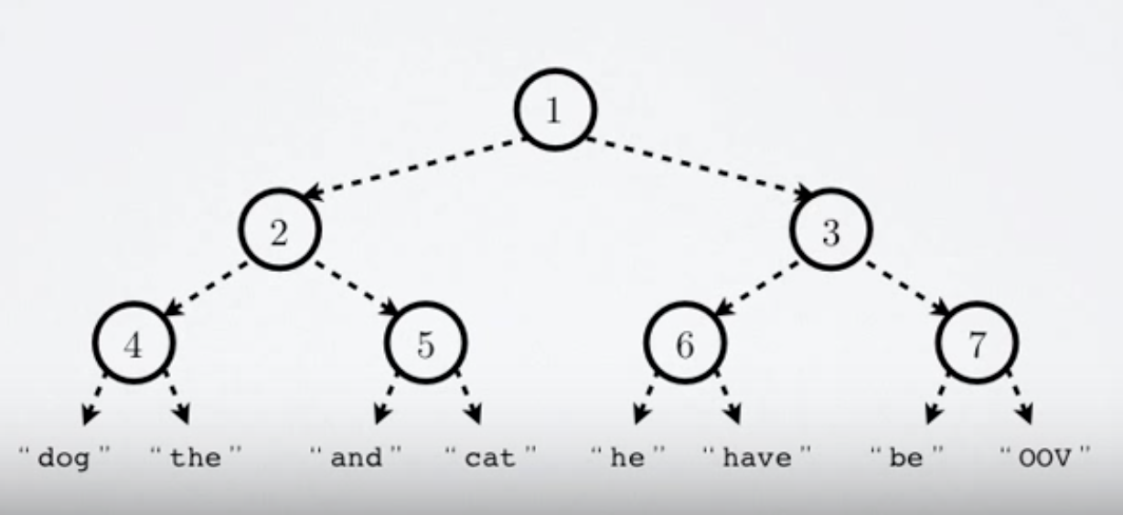
Figure 3: Hierarchical Softmax Tree. (Source)

At each node in the tree starting from the root, we would like to predict the probability of branching right given the observed context. Therefore, in the above tree, if we would like to compute the probability of observing the word “cat” given a certain context, we would define it as the product of going left at node 1, then going right at node 2, and then again going right at node 5 (conditioned on the context).

The actual computation to determine the probability of a word is done by taking the output of the previous layer, applying a set of node-specific weights and biases to it, and running that result through a non-linearity (often sigmoidal). The following image is an illustration of the process of computing the probability of the word “cat” given an observed context:

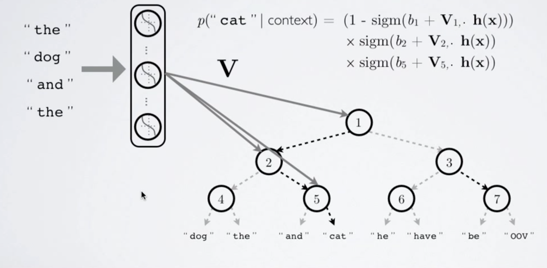
Figure 4: Hierarchical Softmax Computation. (Source)

Here, \(V\) is our matrix of weights connecting the outputs of our previous layer (denoted by \(h(x)\)) to our hierarchical layer, and the probabiltiy of branching right at a certain node is given by \(\sigma(h(x)W_n + b_n)\). The probability of observing a particular word, then is just the product of the branches that lead to it.

In the above image, we also notice that in a vocabulary of 8 words, we only needed 3 computations to approximate the softmax computation as opposed to 8. More generally, hierarchical softmax greatly reduces our computation time to \(log_2(n)\) where \(n\) is our vocabulary size, compared to linear time for the traditional softmax approach. However, this speedup is only useful for training when we don’t need to know the full probability distribution. In settings where we wish to emit the most likely word given a context (for example, in sentence generation), we’d still need to compute the probability of all of the words given the context, resulting in no speed up (although some methods such as pruning when the probability of a certain word quickly tends to zero can certainly increase efficiency).

Negative Sampling and Noise Contrastive Estimation

Multinomial softmax regression is expensive when we are computing softmax across many different classes (each word essentially denotes a separate class). The core idea of Noise Contrastive Estimation (NCE) is to convert a multiclass classification problem into one of binary classification via logistic regression, while still retaining the quality of word vectors learned. With NCE, word vectors are no longer learned by attempting to predict the context words from the target word. Instead we learn word vectors by learning how to distinguish true pairs of (target, context) words from corrupted (target, random word from vocabulary) pairs. The idea is that if a model can distinguish between actual pairs of target and context words from random noise, then good word vectors will be learned.

Specifically, for each positive sample (ie, true target/context pair) we present the model with \(k\) negative samples drawn from a noise distribution. For small to average size training datasets, a value for \(k\) between 5 and 20 was recommended, while for very large datasets a smaller value of \(k\) between 2 and 5 suffices. Our model only has a single output node, which predicts whether the pair was just random noise or actually a valid target/context pair. The noise distribution itself is a free parameter, but the paper found that the unigram distribution raised to the power \(3/4\) worked better than other distributions, such as the unigram and uniform distributions.

The main differences between NCE and Negative sampling is the choice of distribution - the paper used a distribution (discussed above) that sampled less frequently occuring words more often. Moreover, NCE approximately minimizes the log probability across the entire corpus (so it is a good approximation of softmax regression), but this does not hold for negative sampling (but negative sampling still learns quality word vectors).

Practical Considerations

Implementing Softmax: If you’re implementing your own softmax function, it’s important to consider overflow issues. Specifically, the computation \(\sum_i e^{z_i}\) can easily overflow, leading to NaN values while training. To resolve this issue, we can instead compute the equivalent \(\frac{e^{z_i + k}}{\sum_i e^{z_i + k}}\) and set \(k = - max z\) so that the largest exponent is zero, avoiding overflow issues.

Subsampling of frequent words: We don’t get much information from very frequent words such as “the”, “it”, and the like. There will be many more pairs of (the, French) as opposed to (France, French) but we’re more interested in the latter pair. Therefore, it would be useful to subsample some of the more frequent words. We would also like to do this proportionally: very common words are sampled out with high probability, and uncommon words are not sampled out.

In order to do this, the paper defines the probability of discarding a particular word as \(p(w_i) = 1 - \frac{t}{freq(w_i)}\) where \(t\) is an arbitrary constant, taken in the paper to be \(10^{-5}\). This discarding function will cause words that appear with a frequency greater than \(t\) to be sampled out with a high probability, while words that appear with a freqeuncy of less than or equal to \(t\) will not be sampled out. For example, if \(t = 10^{-5}\) and a particular word covers \(0.1%\) of the corpus, then each instance of that word will be discarded from the training corpus with probability \(0.9\).

Conclusion

We have discussed language models including the bag of words model, the n-gram model, and the word2vec model along with changes to the softmax layer in order to more efficiently compute word embeddings. The paper presented empirical results that indicated that negative sampling outperforms hierarchical softmax and (slightly) outperforms NCE on analogical reasoning tasks. Overall, word2vec is one of the most commonly used models for learning dense word embeddings to represent words, and these vectors have several interesting properties (such as additive compositionality). Once these word vectors are learned, they can be a more powerful representation than the typical one-hot encodings when used as inputs into RNNs/LSTMs for applications such as machine translation or sentiment analysis. Thanks for reading! A discussion on Hacker News can be found here.

Sources

• Distributed Representations of Words and Phrases - the main paper discussed.
• Hierarchical Output Layer Video by Hugo Larochelle - an excellent video going into great detail about hierarchical softmax.
• Word2Vec explained - a meta-paper explaining the word2vec paper
• Chris McCormick’s Word2Vec Tutorial
• Stephan Gouws’s Quora answer on Hierarchical Softmax - an insightful answer about the hierarchical output layer
• Word Embeddings Post by Sebastian Ruder - an informative post covering word embeddings and language modelling.
• Efficient estimation of word representations another key word2vec paper discussing the differences (both from an architecture perspective and empirical results) of the bag of words, skip-gram, and word2vec models.